Generative Adversarial Networks

Generative adversarial networks (GANs) are a kind of unsupervised machine learning algorithms that are implemented by a system of two neural networks competing against each other in a zero-sum game framework Goodfellow et al.. The generator creates new data instances, while the discriminator analyzes them for authenticity; that is, the discriminator determines if each data instance corresponds to the real training dataset or not.

To summarize, a GAN follows the following steps for an image generating example:

• The generator takes in random numbers and returns an image.
• This generated image is fed into the discriminator together with a batch of images taken from the actual dataset.
• The discriminator takes in both real and fake images and returns probabilities, a number between 0 and 1, with 1 representing a prediction of authenticity and 0 representing fake.
• Update the weights of the competing neural networks.

Python Tutorial to Train a DCGAN

In this tutorial, I’ll walk you through the python code for training a DCGAN. The code given in this tutorial can be executed inside a Google Colab. The working architecture of convolution layers to the Generator of a DCGAN is seen in the image below.

We can see that strided convolutions are used instead of pooling layers and fully-connected layers (e.g., in a CNN) is replaced with G(Z). In the colab, we begin by installing and loading the required libraries s follow.

%tensorflow_version 1.x
!pip3 install mock
!pip3 install tensorflow-gan
!pip3 install tensorflow-datasets==3.2.1
!pip3 install impl

%cd /content
! rm -rf gan-tools
! rm -rf stylegan-lowshot
!git clone --single-branch --depth=1 --branch master https://github.com/hannesdm/gan-tools.git
!git clone --single-branch --depth=1 --branch main https://github.com/hannesdm/stylegan-lowshot.git
%cd gan-tools
from tensorflow import keras
from keras.datasets import mnist
import impl
from impl import *
from core import vis
from core import gan
from core import constraint
import matplotlib.pyplot as plt
plt.rcParams['image.cmap'] = 'gray'
plt.rcParams['axes.grid'] = False

Loading the cifar10 data

In this tutorial, we will use the CIFAR-10 dataset, which consists of 60000 32x32 colour images in 10 classes, with 6000 images per class. Moreover, there are 50000 training images and 10000 test images. We will select a single class of this dataset to model. This can be done by setting the model_class variable to the corresponding class.

model_class = 1
(X_train_original, Y_train), (_, _) = cifar10.load_data()
X_train_single_class = X_train_original[np.where(np.squeeze(Y_train) == model_class)]
X_train = X_train_single_class / 127.5 - 1.

In the Figure below, few images of the selected class are shown.

Train the DCGAN

The following code will train a GAN. This training can be controlled by the following parameters:

• batches: The number of batches the GAN should train on.
• batch_size: The size of each batch.
• plot_interval: After how many batches the generator should be sampled and the images shown.

The default parameters may be kept. Make sure to train the GAN for a sufficient amount of time in order to see realistic samples. At any point, the training may be stopped by clicking on the stop button or on ‘interrupt execution’ in the runtime menu at the top of the page. In the same menu, the runtime type should also be changed to ‘GPU’. This will speed up the training of the models. We will train the DCGAN for 20000 batches. The code below will train the DCGAN.

gan = cifar10_dcgan()
gan.train_random_batches(X_train, batches = 20000, batch_size=32, plot_interval = 50)
vis.show_gan_image_predictions(gan, 32)

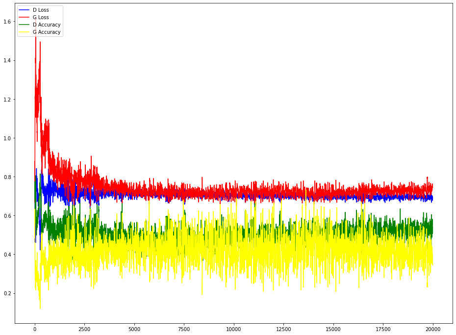
During the training, we can see how the loss and accuracy of the Discriminator and Generator changes. When training is initiated, the Discriminator accuracy is high and Generator loss is also very high. During the training, the Generator improves, therefore, the error gets smaller and that has an impact on the accuracy of the Discriminator, which gets smaller.

The following code will plot the loss and accuracy of the Discriminator and Generator.

def moving_average(a, n=10) :
    s = np.cumsum(a, dtype=float)
    s[n:] = s[n:] - s[:-n]
    return s[n - 1:] / n


plt.figure(figsize=(16, 12))
plt.plot(moving_average(gan.d_losses), c="blue", label="D Loss")
plt.plot(moving_average(gan.g_losses), c="red", label="G Loss")
plt.plot(moving_average(gan.d_accs), c="green", label="D Accuracy")
plt.plot(moving_average(gan.g_accs), c="yellow", label="G Accuracy")
plt.legend(loc="upper left")
plt.show()

The plot below shows that the loss and accuracy of the Discriminator and Generator balance out, as both models improve in parallel.

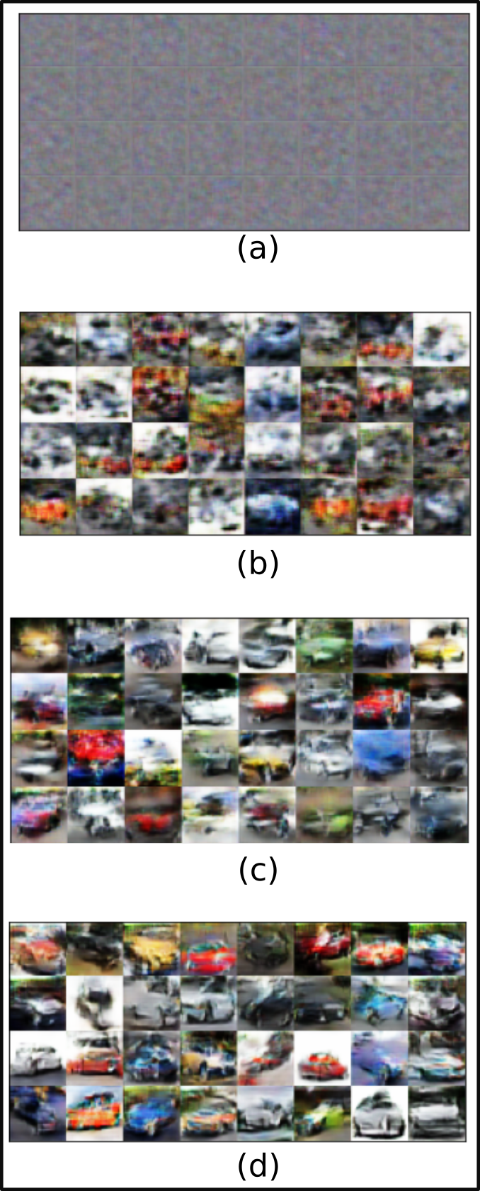
The following figure shows the images of the GAN during the start (a), middle (b and c) and at the end (d) of the training. After the training completes, the images (d) resemble cars, however, they still remain blurry.

Stability in GANs

Sadly, training a GAN is not always easy. Stability during training is important for both discriminator and generator to learn. Below is a short video (50s) showing the intermediate results of a GAN being trained on mnist. The final result is a phenomenon known as mode collapse.

High Quality Image Generation with StyleGAN

The DCGAN model was an important point in the history of generative adversarial networks. However, these models have difficulty with high resolution images and have long been passed by the current state of the art.

State of the art models for high resolution image generation, such as BigGAN and StyleGAN, can generate new images with high fidelity of e.g. 1024x1024 image data sets. The trade-off is that these models can require weeks to train even with the best GPUs and/or TPUs available. Nonetheless, A special setting called Few-shot learning can be used for training generative models learning where one attempts to create a model that generalizes well on as few samples as possible. This setting allows the power of the state of the art models to be demonstrated while still being able to be trained in a reasonable time.

StyleGAN few-shot

The following script allows you to train a StyleGAN with differentiable augmentations on your own data. Few-shot models work best with uniform, clean data where the object takes up the majority of the image. To the left of Google Colab, click the folder icon on the sidebar, create a new folder in the file explorer and upload your images into it. It’s recommended to have at least 100 images. Next, replace the placeholder in the command below with the link to your uploaded folder (e.g. /content/mydata) and execute the command. It’s recommended to try out different types of data to see what works and what doesn’t. Alternatively, replace the placeholder by the name of one of the pre-existing data sets:

• 100-shot-obama
• 100-shot-grumpy_cat
• 100-shot-panda
• 100-shot-bridge_of_sighs
• 100-shot-temple_of_heaven
• 100-shot-wuzhen

The script will output intermediate images while training. More full quality samples can be found in the /content/stylegan-lowshot/results folder. Take note that it can take multiple hours before reasonable images start to be generated even when working with these very small data sets.

%cd /content/stylegan-lowshot
%run run_low_shot.py --dataset=/content/mydata --num-gpus=1 --resolution=128 --show-samples-every=1